Data Transforms

data_path = '/home/naji/Desktop/github-repos/machine-learning/nbs/0-datasets/data/'

Scale Numerical Data

Numerical Data Scaling Methods

from pandas import read_csv, DataFrame
from numpy import asarray, mean, std
from sklearn.preprocessing import LabelEncoder, MinMaxScaler, StandardScaler
from sklearn.neighbors import KNeighborsClassifier
from sklearn.model_selection import RepeatedStratifiedKFold, cross_val_score, train_test_split
from sklearn.neighbors import KNeighborsClassifier
from sklearn.pipeline import Pipeline
from matplotlib import pyplot

Data Normalization

from sklearn.preprocessing import MinMaxScaler

data = asarray([[100, 0.001],
                [8, 0.05],
                [50, 0.005],
                [88, 0.07],
                [4, 0.1]])

print(data)

[[1.0e+02 1.0e-03]
 [8.0e+00 5.0e-02]
 [5.0e+01 5.0e-03]
 [8.8e+01 7.0e-02]
 [4.0e+00 1.0e-01]]

scaler = MinMaxScaler()

scaled = scaler.fit_transform(data)

print(scaled)

[[1.         0.        ]
 [0.04166667 0.49494949]
 [0.47916667 0.04040404]
 [0.875      0.6969697 ]
 [0.         1.        ]]

Data Standardization

from sklearn.preprocessing import StandardScaler

data = asarray([[100, 0.001],
                [8, 0.05],
                [50, 0.005],
                [88, 0.07],
                [4, 0.1]])

scaler = StandardScaler()

scaled = scaler.fit_transform(data)

print(scaled)

[[ 1.26398112 -1.16389967]
 [-1.06174414  0.12639634]
 [ 0.         -1.05856939]
 [ 0.96062565  0.65304778]
 [-1.16286263  1.44302493]]

Diabetes Dataset

df = read_csv(data_path + 'pima-indians-diabetes.csv', header=None)
df

	0	1	2	3	4	5	6	7	8
0	6	148	72	35	0	33.6	0.627	50	1
1	1	85	66	29	0	26.6	0.351	31	0
2	8	183	64	0	0	23.3	0.672	32	1
3	1	89	66	23	94	28.1	0.167	21	0
4	0	137	40	35	168	43.1	2.288	33	1
...	...	...	...	...	...	...	...	...	...
763	10	101	76	48	180	32.9	0.171	63	0
764	2	122	70	27	0	36.8	0.340	27	0
765	5	121	72	23	112	26.2	0.245	30	0
766	1	126	60	0	0	30.1	0.349	47	1
767	1	93	70	31	0	30.4	0.315	23	0

768 rows × 9 columns

df.shape

(768, 9)

print(df.describe())

                0           1           2  ...           6           7           8
count  768.000000  768.000000  768.000000  ...  768.000000  768.000000  768.000000
mean     3.845052  120.894531   69.105469  ...    0.471876   33.240885    0.348958
std      3.369578   31.972618   19.355807  ...    0.331329   11.760232    0.476951
min      0.000000    0.000000    0.000000  ...    0.078000   21.000000    0.000000
25%      1.000000   99.000000   62.000000  ...    0.243750   24.000000    0.000000
50%      3.000000  117.000000   72.000000  ...    0.372500   29.000000    0.000000
75%      6.000000  140.250000   80.000000  ...    0.626250   41.000000    1.000000
max     17.000000  199.000000  122.000000  ...    2.420000   81.000000    1.000000

[8 rows x 9 columns]

fig = df.hist(xlabelsize=4, ylabelsize=4)
[x.title.set_size(4) for x in fig.ravel()]
pyplot.show()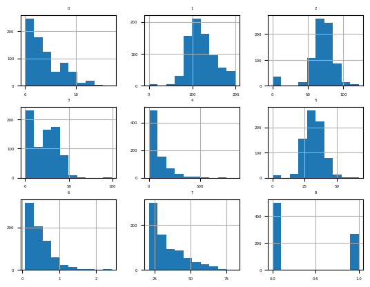

data = df.values

X, y = data[:, :-1], data[:, -1]

X = X.astype('float32')

y = LabelEncoder().fit_transform(y.astype('str'))

model = KNeighborsClassifier()

cv = RepeatedStratifiedKFold(n_splits=10, n_repeats=3, random_state=1)

scores = cross_val_score(model, X, y, scoring='accuracy', cv=cv)

print(f'Accuracy: {mean(scores):0.3f}  {std(scores):0.3f}')

Accuracy: 0.717  0.040

MinMaxScaler Transform

df = read_csv(data_path + 'pima-indians-diabetes.csv', header=None)

data = df.values

trans = MinMaxScaler()

data = trans.fit_transform(data)

df = DataFrame(data)

print(df.describe())

                0           1           2  ...           6           7           8
count  768.000000  768.000000  768.000000  ...  768.000000  768.000000  768.000000
mean     0.226180    0.607510    0.566438  ...    0.168179    0.204015    0.348958
std      0.198210    0.160666    0.158654  ...    0.141473    0.196004    0.476951
min      0.000000    0.000000    0.000000  ...    0.000000    0.000000    0.000000
25%      0.058824    0.497487    0.508197  ...    0.070773    0.050000    0.000000
50%      0.176471    0.587940    0.590164  ...    0.125747    0.133333    0.000000
75%      0.352941    0.704774    0.655738  ...    0.234095    0.333333    1.000000
max      1.000000    1.000000    1.000000  ...    1.000000    1.000000    1.000000

[8 rows x 9 columns]

fig = df.hist(xlabelsize=4, ylabelsize=4)
[x.title.set_size(4) for x in fig.ravel()]
pyplot.show()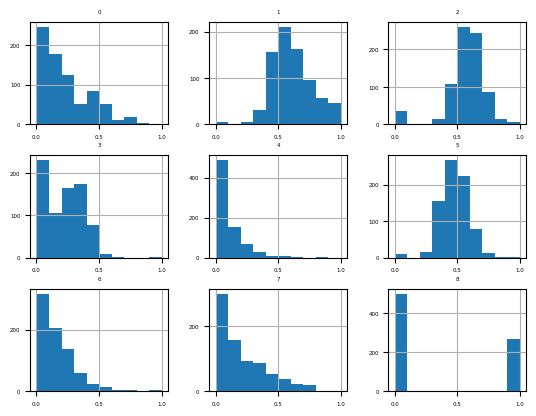

Train the model

df = read_csv(data_path + 'pima-indians-diabetes.csv', header=None)

data = df.values

X, y = data[:, :-1], data[:, -1]

X = X.astype('float32')
y = LabelEncoder().fit_transform(y.astype('str'))

trans = MinMaxScaler()

model = KNeighborsClassifier()

pipeline = Pipeline(steps=[('t', trans), ('m', model)])

cv = RepeatedStratifiedKFold(n_splits=10, n_repeats=3, random_state=1)

scores = cross_val_score(pipeline, X, y, scoring='accuracy', cv=cv)

print(f'Accuracy: {mean(scores):0.3f}, {std(scores):.3f}')

Accuracy: 0.739, 0.053

StandardScaler Transform

df = read_csv(data_path + 'pima-indians-diabetes.csv', header=None)

data = df.values[:, :-1]

trans = StandardScaler()

data = trans.fit_transform(data)

df = DataFrame(data)

print(df.describe())

                  0             1  ...             6             7
count  7.680000e+02  7.680000e+02  ...  7.680000e+02  7.680000e+02
mean  -6.476301e-17 -9.251859e-18  ...  2.451743e-16  1.931325e-16
std    1.000652e+00  1.000652e+00  ...  1.000652e+00  1.000652e+00
min   -1.141852e+00 -3.783654e+00  ... -1.189553e+00 -1.041549e+00
25%   -8.448851e-01 -6.852363e-01  ... -6.889685e-01 -7.862862e-01
50%   -2.509521e-01 -1.218877e-01  ... -3.001282e-01 -3.608474e-01
75%    6.399473e-01  6.057709e-01  ...  4.662269e-01  6.602056e-01
max    3.906578e+00  2.444478e+00  ...  5.883565e+00  4.063716e+00

[8 rows x 8 columns]

fig = df.hist(xlabelsize=4, ylabelsize=4)
[x.title.set_size(4) for x in fig.ravel()]
pyplot.show()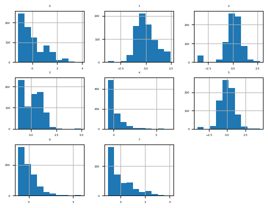

Train the model

df = read_csv(data_path + 'pima-indians-diabetes.csv', header=None)

data = df.values

X, y = data[:, :-1], data[:, -1]

X = X.astype('float32')

y = LabelEncoder().fit_transform(y.astype('str'))

trans = StandardScaler()

model = KNeighborsClassifier()

pipeline = Pipeline(steps=[('t', trans), ('m', model)])

cv = RepeatedStratifiedKFold(n_splits=10, n_repeats=3, random_state=1)

scores = cross_val_score(pipeline, X, y, scoring='accuracy', cv=cv)

print(f'Accuracy: {mean(scores):.3f}  {std(scores):.3f}')

Accuracy: 0.741  0.050

Scale Data With Outliers

IQR Robust Scaler Transform

from sklearn.preprocessing import RobustScaler

df = read_csv(data_path + 'pima-indians-diabetes.csv', header=None)

data = df.values[:, :-1]

trans = RobustScaler()

data = trans.fit_transform(data)

df = DataFrame(data)

print(df.describe())

                0           1           2  ...           5           6           7
count  768.000000  768.000000  768.000000  ...  768.000000  768.000000  768.000000
mean     0.169010    0.094413   -0.160807  ...   -0.000798    0.259807    0.249464
std      0.673916    0.775094    1.075323  ...    0.847759    0.866219    0.691778
min     -0.600000   -2.836364   -4.000000  ...   -3.440860   -0.769935   -0.470588
25%     -0.400000   -0.436364   -0.555556  ...   -0.505376   -0.336601   -0.294118
50%      0.000000    0.000000    0.000000  ...    0.000000    0.000000    0.000000
75%      0.600000    0.563636    0.444444  ...    0.494624    0.663399    0.705882
max      2.800000    1.987879    2.777778  ...    3.774194    5.352941    3.058824

[8 rows x 8 columns]

fig = df.hist(xlabelsize=4, ylabelsize=4)
[x.title.set_size(4) for x in fig.ravel()]
pyplot.show()

Train the model

df = read_csv(data_path + 'pima-indians-diabetes.csv', header=None)

data = df.values

X, y = data[:, :-1], data[:, -1]

X = X.astype('float32')

y = LabelEncoder().fit_transform(y.astype('str'))

trans = RobustScaler()

model = KNeighborsClassifier()

pipeline = Pipeline(steps=[('t', trans), ('m', model)])

cv = RepeatedStratifiedKFold(n_splits=10, n_repeats=3, random_state=1)

scores = cross_val_score(pipeline, X, y, scoring='accuracy', cv=cv)

print(f'Accuracy: {mean(scores):.3f}  {std(scores):.3f}')

Accuracy: 0.734  0.044

Explore Robust Scaler Range

def get_dataset():
    df = read_csv(data_path + 'pima-indians-diabetes.csv', header=None)
    data = df.values
    X, y = data[:, :-1], data[:, -1]
    X = X.astype('float32')
    y = LabelEncoder().fit_transform(y.astype('str'))
    return X, y

def get_models():
    models = dict()
    for value in [1, 5, 10, 20, 25, 30]:
        trans = RobustScaler(quantile_range=(value, 100-value))
        model = KNeighborsClassifier()
        models[str(value)] = Pipeline(steps=[('t', trans), ('m', model)])
    return models

def evaluate_model(model, X, y):
    cv = RepeatedStratifiedKFold(n_splits=10, n_repeats=3, random_state=1)
    scores = cross_val_score(model, X, y, scoring='accuracy', cv=cv)
    return scores

x, y = get_dataset()

models = get_models()

results, names = list(), list()

for name, model in models.items():
    scores = evaluate_model(model, X, y)
    results.append(scores)
    names.append(name)
    print(f'{name:} {mean(scores):.3f} {std(scores):.3f}')

1 0.734 0.054
5 0.736 0.051
10 0.739 0.047
20 0.734 0.050
25 0.734 0.044
30 0.735 0.042

pyplot.boxplot(results, labels=names, showmeans=True)
pyplot.show()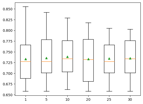

Encode Categorical Data

Encoding Categorical Data

Ordinal Encoding

from sklearn.preprocessing import OrdinalEncoder

data = asarray([['red'], ['green'], ['blue']])

print(data)

[['red']
 ['green']
 ['blue']]

encoder = OrdinalEncoder()

result = encoder.fit_transform(data)

print(result)

[[2.]
 [1.]
 [0.]]

One Hot Encoding

from sklearn.preprocessing import OneHotEncoder

data = asarray([['red'], ['green'], ['blue']])

print(data)

[['red']
 ['green']
 ['blue']]

encoder = OneHotEncoder(sparse=False)

onehot = encoder.fit_transform(data)

print(onehot)

[[0. 0. 1.]
 [0. 1. 0.]
 [1. 0. 0.]]

Dummy Variable Encoding

from sklearn.preprocessing import OneHotEncoder

data = asarray([['red'],['green'],['blue']])
print(data)

[['red']
 ['green']
 ['blue']]

encoder = OneHotEncoder(drop='first', sparse=False)

onehot = encoder.fit_transform(data)
print(onehot)

[[0. 1.]
 [1. 0.]
 [0. 0.]]

Breast Cancer Dataset

df = read_csv(data_path + 'breast-cancer.csv', header=None)
df

	0	1	2	3	4	5	6	7	8	9
0	'40-49'	'premeno'	'15-19'	'0-2'	'yes'	'3'	'right'	'left_up'	'no'	'recurrence-events'
1	'50-59'	'ge40'	'15-19'	'0-2'	'no'	'1'	'right'	'central'	'no'	'no-recurrence-events'
2	'50-59'	'ge40'	'35-39'	'0-2'	'no'	'2'	'left'	'left_low'	'no'	'recurrence-events'
3	'40-49'	'premeno'	'35-39'	'0-2'	'yes'	'3'	'right'	'left_low'	'yes'	'no-recurrence-events'
4	'40-49'	'premeno'	'30-34'	'3-5'	'yes'	'2'	'left'	'right_up'	'no'	'recurrence-events'
...	...	...	...	...	...	...	...	...	...	...
281	'50-59'	'ge40'	'30-34'	'6-8'	'yes'	'2'	'left'	'left_low'	'no'	'no-recurrence-events'
282	'50-59'	'premeno'	'25-29'	'3-5'	'yes'	'2'	'left'	'left_low'	'yes'	'no-recurrence-events'
283	'30-39'	'premeno'	'30-34'	'6-8'	'yes'	'2'	'right'	'right_up'	'no'	'no-recurrence-events'
284	'50-59'	'premeno'	'15-19'	'0-2'	'no'	'2'	'right'	'left_low'	'no'	'no-recurrence-events'
285	'50-59'	'ge40'	'40-44'	'0-2'	'no'	'3'	'left'	'right_up'	'no'	'no-recurrence-events'

286 rows × 10 columns

data = df.values

X = data[:, :-1].astype(str)
y = data[:, -1].astype(str)

print('Input', X.shape)

Input (286, 9)

print('Output', y.shape)

Output (286,)

OrdinalEncoder Transform

ordinal_encoder = OrdinalEncoder()

X = ordinal_encoder.fit_transform(X)

label_encoder = LabelEncoder()

y = label_encoder.fit_transform(y)

print('Input', X.shape)

Input (286, 9)

X[:10, :]

array([[2., 2., 2., 0., 1., 2., 1., 2., 0.],
       [3., 0., 2., 0., 0., 0., 1., 0., 0.],
       [3., 0., 6., 0., 0., 1., 0., 1., 0.],
       [2., 2., 6., 0., 1., 2., 1., 1., 1.],
       [2., 2., 5., 4., 1., 1., 0., 4., 0.],
       [3., 2., 4., 4., 0., 1., 1., 2., 1.],
       [3., 0., 7., 0., 0., 2., 0., 2., 0.],
       [2., 2., 1., 0., 0., 1., 0., 2., 0.],
       [2., 2., 0., 0., 0., 1., 1., 3., 0.],
       [2., 0., 7., 2., 1., 1., 1., 2., 1.]])

print('Output', y.shape)

Output (286,)

y[:10]

array([1, 0, 1, 0, 1, 0, 0, 0, 0, 0])

Training a model

from sklearn.linear_model import LogisticRegression
from sklearn.metrics import accuracy_score

df = read_csv(data_path + 'breast-cancer.csv', header=None)

data = df.values

X = data[:, :-1].astype(str)
y = data[:, -1].astype(str)

X_train, X_test, y_train, y_test = train_test_split(X, y, test_size=.33, random_state=1)

ordinal_encoder = OrdinalEncoder()

ordinal_encoder.fit(X_train)

OrdinalEncoder()

In a Jupyter environment, please rerun this cell to show the HTML representation or trust the notebook.
On GitHub, the HTML representation is unable to render, please try loading this page with nbviewer.org.

X_train = ordinal_encoder.transform(X_train)
X_test = ordinal_encoder.transform(X_test)

label_encoder = LabelEncoder()

label_encoder.fit(y_train)

LabelEncoder()

y_train = label_encoder.transform(y_train)

y_test = label_encoder.transform(y_test)

model = LogisticRegression()

model.fit(X_train, y_train)

LogisticRegression()

yhat = model.predict(X_test)

accuracy = accuracy_score(y_test, yhat)

print(f'Accuracy: {accuracy*100: .3f}')

Accuracy:  75.789

OneHotEncoder Transform

df = read_csv(data_path + 'breast-cancer.csv', header=None)

data = df.values

X = data[:, :-1].astype(str)
y = data[:, -1].astype(str)

onehot_encoder = OneHotEncoder(sparse=False)

X = onehot_encoder.fit_transform(X)

label_encoder = LabelEncoder()

y = label_encoder.fit_transform(y)

print('Input', X.shape)

Input (286, 43)

print(X[:5, :])

[[0. 0. 1. 0. 0. 0. 0. 0. 1. 0. 0. 1. 0. 0. 0. 0. 0. 0. 0. 0. 1. 0. 0. 0.
  0. 0. 0. 0. 1. 0. 0. 0. 1. 0. 1. 0. 0. 1. 0. 0. 0. 1. 0.]
 [0. 0. 0. 1. 0. 0. 1. 0. 0. 0. 0. 1. 0. 0. 0. 0. 0. 0. 0. 0. 1. 0. 0. 0.
  0. 0. 0. 1. 0. 0. 1. 0. 0. 0. 1. 1. 0. 0. 0. 0. 0. 1. 0.]
 [0. 0. 0. 1. 0. 0. 1. 0. 0. 0. 0. 0. 0. 0. 0. 1. 0. 0. 0. 0. 1. 0. 0. 0.
  0. 0. 0. 1. 0. 0. 0. 1. 0. 1. 0. 0. 1. 0. 0. 0. 0. 1. 0.]
 [0. 0. 1. 0. 0. 0. 0. 0. 1. 0. 0. 0. 0. 0. 0. 1. 0. 0. 0. 0. 1. 0. 0. 0.
  0. 0. 0. 0. 1. 0. 0. 0. 1. 0. 1. 0. 1. 0. 0. 0. 0. 0. 1.]
 [0. 0. 1. 0. 0. 0. 0. 0. 1. 0. 0. 0. 0. 0. 1. 0. 0. 0. 0. 0. 0. 0. 0. 0.
  1. 0. 0. 0. 1. 0. 0. 1. 0. 1. 0. 0. 0. 0. 0. 1. 0. 1. 0.]]

Train the model

df = read_csv(data_path + 'breast-cancer.csv', header=None)

data = df.values

X = data[:, :-1].astype(str)
y = data[:, -1].astype(str)

X_train, X_test, y_train, y_test = train_test_split(X, y, test_size=0.33, random_state=1)

onehot_encoder = OneHotEncoder()

onehot_encoder.fit(X_train)

OneHotEncoder()

X_train = onehot_encoder.transform(X_train)
X_test = onehot_encoder.transform(X_test)

label_encoder = LabelEncoder()

label_encoder.fit(y_train)

LabelEncoder()

y_train = label_encoder.transform(y_train)

y_test = label_encoder.transform(y_test)

model = LogisticRegression()

model.fit(X_train, y_train)

LogisticRegression()

yhat = model.predict(X_test)

accuracy = accuracy_score(y_test, yhat)

print(f'Accuracy: {accuracy*100: .3f}')

Accuracy:  70.526

How to Make Distributions More Gaussian

Power Transforms

from numpy import exp 
from numpy.random import randn
from sklearn.preprocessing import PowerTransformer

data = randn(1000)

data = exp(data)

pyplot.hist(data, bins=25)
pyplot.show()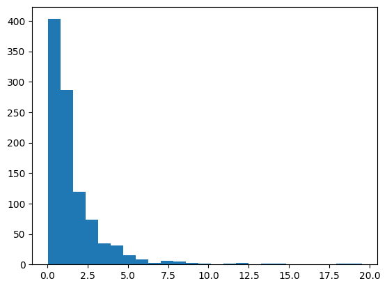

data = data.reshape(len(data), 1)

power = PowerTransformer(method='yeo-johnson', standardize=True)

data_trans = power.fit_transform(data)

pyplot.hist(data_trans, bins=25)
pyplot.show()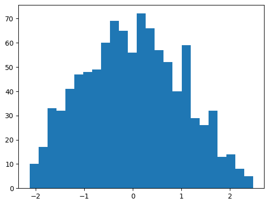

Sonar Dataset

from sklearn.preprocessing import LabelEncoder

df = read_csv(data_path + 'sonar.csv', header=None)

df

	0	1	2	3	4	5	6	7	8	9	10	11	12	13	14	15	16	17	18	19	20	21	22	23	24	25	26	27	28	29	30	31	32	33	34	35	36	37	38	39	40	41	42	43	44	45	46	47	48	49	50	51	52	53	54	55	56	57	58	59	60
0	0.0200	0.0371	0.0428	0.0207	0.0954	0.0986	0.1539	0.1601	0.3109	0.2111	0.1609	0.1582	0.2238	0.0645	0.0660	0.2273	0.3100	0.2999	0.5078	0.4797	0.5783	0.5071	0.4328	0.5550	0.6711	0.6415	0.7104	0.8080	0.6791	0.3857	0.1307	0.2604	0.5121	0.7547	0.8537	0.8507	0.6692	0.6097	0.4943	0.2744	0.0510	0.2834	0.2825	0.4256	0.2641	0.1386	0.1051	0.1343	0.0383	0.0324	0.0232	0.0027	0.0065	0.0159	0.0072	0.0167	0.0180	0.0084	0.0090	0.0032	R
1	0.0453	0.0523	0.0843	0.0689	0.1183	0.2583	0.2156	0.3481	0.3337	0.2872	0.4918	0.6552	0.6919	0.7797	0.7464	0.9444	1.0000	0.8874	0.8024	0.7818	0.5212	0.4052	0.3957	0.3914	0.3250	0.3200	0.3271	0.2767	0.4423	0.2028	0.3788	0.2947	0.1984	0.2341	0.1306	0.4182	0.3835	0.1057	0.1840	0.1970	0.1674	0.0583	0.1401	0.1628	0.0621	0.0203	0.0530	0.0742	0.0409	0.0061	0.0125	0.0084	0.0089	0.0048	0.0094	0.0191	0.0140	0.0049	0.0052	0.0044	R
2	0.0262	0.0582	0.1099	0.1083	0.0974	0.2280	0.2431	0.3771	0.5598	0.6194	0.6333	0.7060	0.5544	0.5320	0.6479	0.6931	0.6759	0.7551	0.8929	0.8619	0.7974	0.6737	0.4293	0.3648	0.5331	0.2413	0.5070	0.8533	0.6036	0.8514	0.8512	0.5045	0.1862	0.2709	0.4232	0.3043	0.6116	0.6756	0.5375	0.4719	0.4647	0.2587	0.2129	0.2222	0.2111	0.0176	0.1348	0.0744	0.0130	0.0106	0.0033	0.0232	0.0166	0.0095	0.0180	0.0244	0.0316	0.0164	0.0095	0.0078	R
3	0.0100	0.0171	0.0623	0.0205	0.0205	0.0368	0.1098	0.1276	0.0598	0.1264	0.0881	0.1992	0.0184	0.2261	0.1729	0.2131	0.0693	0.2281	0.4060	0.3973	0.2741	0.3690	0.5556	0.4846	0.3140	0.5334	0.5256	0.2520	0.2090	0.3559	0.6260	0.7340	0.6120	0.3497	0.3953	0.3012	0.5408	0.8814	0.9857	0.9167	0.6121	0.5006	0.3210	0.3202	0.4295	0.3654	0.2655	0.1576	0.0681	0.0294	0.0241	0.0121	0.0036	0.0150	0.0085	0.0073	0.0050	0.0044	0.0040	0.0117	R
4	0.0762	0.0666	0.0481	0.0394	0.0590	0.0649	0.1209	0.2467	0.3564	0.4459	0.4152	0.3952	0.4256	0.4135	0.4528	0.5326	0.7306	0.6193	0.2032	0.4636	0.4148	0.4292	0.5730	0.5399	0.3161	0.2285	0.6995	1.0000	0.7262	0.4724	0.5103	0.5459	0.2881	0.0981	0.1951	0.4181	0.4604	0.3217	0.2828	0.2430	0.1979	0.2444	0.1847	0.0841	0.0692	0.0528	0.0357	0.0085	0.0230	0.0046	0.0156	0.0031	0.0054	0.0105	0.0110	0.0015	0.0072	0.0048	0.0107	0.0094	R
...	...	...	...	...	...	...	...	...	...	...	...	...	...	...	...	...	...	...	...	...	...	...	...	...	...	...	...	...	...	...	...	...	...	...	...	...	...	...	...	...	...	...	...	...	...	...	...	...	...	...	...	...	...	...	...	...	...	...	...	...	...
203	0.0187	0.0346	0.0168	0.0177	0.0393	0.1630	0.2028	0.1694	0.2328	0.2684	0.3108	0.2933	0.2275	0.0994	0.1801	0.2200	0.2732	0.2862	0.2034	0.1740	0.4130	0.6879	0.8120	0.8453	0.8919	0.9300	0.9987	1.0000	0.8104	0.6199	0.6041	0.5547	0.4160	0.1472	0.0849	0.0608	0.0969	0.1411	0.1676	0.1200	0.1201	0.1036	0.1977	0.1339	0.0902	0.1085	0.1521	0.1363	0.0858	0.0290	0.0203	0.0116	0.0098	0.0199	0.0033	0.0101	0.0065	0.0115	0.0193	0.0157	M
204	0.0323	0.0101	0.0298	0.0564	0.0760	0.0958	0.0990	0.1018	0.1030	0.2154	0.3085	0.3425	0.2990	0.1402	0.1235	0.1534	0.1901	0.2429	0.2120	0.2395	0.3272	0.5949	0.8302	0.9045	0.9888	0.9912	0.9448	1.0000	0.9092	0.7412	0.7691	0.7117	0.5304	0.2131	0.0928	0.1297	0.1159	0.1226	0.1768	0.0345	0.1562	0.0824	0.1149	0.1694	0.0954	0.0080	0.0790	0.1255	0.0647	0.0179	0.0051	0.0061	0.0093	0.0135	0.0063	0.0063	0.0034	0.0032	0.0062	0.0067	M
205	0.0522	0.0437	0.0180	0.0292	0.0351	0.1171	0.1257	0.1178	0.1258	0.2529	0.2716	0.2374	0.1878	0.0983	0.0683	0.1503	0.1723	0.2339	0.1962	0.1395	0.3164	0.5888	0.7631	0.8473	0.9424	0.9986	0.9699	1.0000	0.8630	0.6979	0.7717	0.7305	0.5197	0.1786	0.1098	0.1446	0.1066	0.1440	0.1929	0.0325	0.1490	0.0328	0.0537	0.1309	0.0910	0.0757	0.1059	0.1005	0.0535	0.0235	0.0155	0.0160	0.0029	0.0051	0.0062	0.0089	0.0140	0.0138	0.0077	0.0031	M
206	0.0303	0.0353	0.0490	0.0608	0.0167	0.1354	0.1465	0.1123	0.1945	0.2354	0.2898	0.2812	0.1578	0.0273	0.0673	0.1444	0.2070	0.2645	0.2828	0.4293	0.5685	0.6990	0.7246	0.7622	0.9242	1.0000	0.9979	0.8297	0.7032	0.7141	0.6893	0.4961	0.2584	0.0969	0.0776	0.0364	0.1572	0.1823	0.1349	0.0849	0.0492	0.1367	0.1552	0.1548	0.1319	0.0985	0.1258	0.0954	0.0489	0.0241	0.0042	0.0086	0.0046	0.0126	0.0036	0.0035	0.0034	0.0079	0.0036	0.0048	M
207	0.0260	0.0363	0.0136	0.0272	0.0214	0.0338	0.0655	0.1400	0.1843	0.2354	0.2720	0.2442	0.1665	0.0336	0.1302	0.1708	0.2177	0.3175	0.3714	0.4552	0.5700	0.7397	0.8062	0.8837	0.9432	1.0000	0.9375	0.7603	0.7123	0.8358	0.7622	0.4567	0.1715	0.1549	0.1641	0.1869	0.2655	0.1713	0.0959	0.0768	0.0847	0.2076	0.2505	0.1862	0.1439	0.1470	0.0991	0.0041	0.0154	0.0116	0.0181	0.0146	0.0129	0.0047	0.0039	0.0061	0.0040	0.0036	0.0061	0.0115	M

208 rows × 61 columns

df.shape

(208, 61)

df.describe()

	0	1	2	3	4	5	6	7	8	9	10	11	12	13	14	15	16	17	18	19	20	21	22	23	24	25	26	27	28	29	30	31	32	33	34	35	36	37	38	39	40	41	42	43	44	45	46	47	48	49	50	51	52	53	54	55	56	57	58	59
count	208.000000	208.000000	208.000000	208.000000	208.000000	208.000000	208.000000	208.000000	208.000000	208.000000	208.000000	208.000000	208.000000	208.000000	208.000000	208.000000	208.000000	208.000000	208.000000	208.000000	208.000000	208.000000	208.000000	208.000000	208.000000	208.000000	208.000000	208.000000	208.000000	208.000000	208.000000	208.000000	208.000000	208.000000	208.000000	208.000000	208.000000	208.000000	208.000000	208.000000	208.000000	208.000000	208.000000	208.000000	208.000000	208.000000	208.000000	208.000000	208.000000	208.000000	208.000000	208.000000	208.000000	208.000000	208.000000	208.000000	208.000000	208.000000	208.000000	208.000000
mean	0.029164	0.038437	0.043832	0.053892	0.075202	0.104570	0.121747	0.134799	0.178003	0.208259	0.236013	0.250221	0.273305	0.296568	0.320201	0.378487	0.415983	0.452318	0.504812	0.563047	0.609060	0.624275	0.646975	0.672654	0.675424	0.699866	0.702155	0.694024	0.642074	0.580928	0.504475	0.439040	0.417220	0.403233	0.392571	0.384848	0.363807	0.339657	0.325800	0.311207	0.289252	0.278293	0.246542	0.214075	0.197232	0.160631	0.122453	0.091424	0.051929	0.020424	0.016069	0.013420	0.010709	0.010941	0.009290	0.008222	0.007820	0.007949	0.007941	0.006507
std	0.022991	0.032960	0.038428	0.046528	0.055552	0.059105	0.061788	0.085152	0.118387	0.134416	0.132705	0.140072	0.140962	0.164474	0.205427	0.232650	0.263677	0.261529	0.257988	0.262653	0.257818	0.255883	0.250175	0.239116	0.244926	0.237228	0.245657	0.237189	0.240250	0.220749	0.213992	0.213237	0.206513	0.231242	0.259132	0.264121	0.239912	0.212973	0.199075	0.178662	0.171111	0.168728	0.138993	0.133291	0.151628	0.133938	0.086953	0.062417	0.035954	0.013665	0.012008	0.009634	0.007060	0.007301	0.007088	0.005736	0.005785	0.006470	0.006181	0.005031
min	0.001500	0.000600	0.001500	0.005800	0.006700	0.010200	0.003300	0.005500	0.007500	0.011300	0.028900	0.023600	0.018400	0.027300	0.003100	0.016200	0.034900	0.037500	0.049400	0.065600	0.051200	0.021900	0.056300	0.023900	0.024000	0.092100	0.048100	0.028400	0.014400	0.061300	0.048200	0.040400	0.047700	0.021200	0.022300	0.008000	0.035100	0.038300	0.037100	0.011700	0.036000	0.005600	0.000000	0.000000	0.000000	0.000000	0.000000	0.000000	0.000000	0.000000	0.000000	0.000800	0.000500	0.001000	0.000600	0.000400	0.000300	0.000300	0.000100	0.000600
25%	0.013350	0.016450	0.018950	0.024375	0.038050	0.067025	0.080900	0.080425	0.097025	0.111275	0.129250	0.133475	0.166125	0.175175	0.164625	0.196300	0.205850	0.242075	0.299075	0.350625	0.399725	0.406925	0.450225	0.540725	0.525800	0.544175	0.531900	0.534775	0.463700	0.411400	0.345550	0.281400	0.257875	0.217575	0.179375	0.154350	0.160100	0.174275	0.173975	0.186450	0.163100	0.158900	0.155200	0.126875	0.094475	0.068550	0.064250	0.045125	0.026350	0.011550	0.008425	0.007275	0.005075	0.005375	0.004150	0.004400	0.003700	0.003600	0.003675	0.003100
50%	0.022800	0.030800	0.034300	0.044050	0.062500	0.092150	0.106950	0.112100	0.152250	0.182400	0.224800	0.249050	0.263950	0.281100	0.281700	0.304700	0.308400	0.368300	0.434950	0.542500	0.617700	0.664900	0.699700	0.698500	0.721100	0.754500	0.745600	0.731900	0.680800	0.607150	0.490350	0.429600	0.391200	0.351050	0.312750	0.321150	0.306300	0.312700	0.283500	0.278050	0.259500	0.245100	0.222550	0.177700	0.148000	0.121350	0.101650	0.078100	0.044700	0.017900	0.013900	0.011400	0.009550	0.009300	0.007500	0.006850	0.005950	0.005800	0.006400	0.005300
75%	0.035550	0.047950	0.057950	0.064500	0.100275	0.134125	0.154000	0.169600	0.233425	0.268700	0.301650	0.331250	0.351250	0.386175	0.452925	0.535725	0.659425	0.679050	0.731400	0.809325	0.816975	0.831975	0.848575	0.872175	0.873725	0.893800	0.917100	0.900275	0.852125	0.735175	0.641950	0.580300	0.556125	0.596125	0.593350	0.556525	0.518900	0.440550	0.434900	0.424350	0.387525	0.384250	0.324525	0.271750	0.231550	0.200375	0.154425	0.120100	0.068525	0.025275	0.020825	0.016725	0.014900	0.014500	0.012100	0.010575	0.010425	0.010350	0.010325	0.008525
max	0.137100	0.233900	0.305900	0.426400	0.401000	0.382300	0.372900	0.459000	0.682800	0.710600	0.734200	0.706000	0.713100	0.997000	1.000000	0.998800	1.000000	1.000000	1.000000	1.000000	1.000000	1.000000	1.000000	1.000000	1.000000	1.000000	1.000000	1.000000	1.000000	1.000000	0.965700	0.930600	1.000000	0.964700	1.000000	1.000000	0.949700	1.000000	0.985700	0.929700	0.899500	0.824600	0.773300	0.776200	0.703400	0.729200	0.552200	0.333900	0.198100	0.082500	0.100400	0.070900	0.039000	0.035200	0.044700	0.039400	0.035500	0.044000	0.036400	0.043900

fig = df.hist(xlabelsize=4, ylabelsize=4)
[x.title.set_size(4) for x in fig.ravel()]
pyplot.show()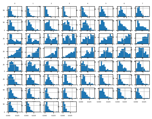

data = df.values

X, y = data[:, :-1], data[:, -1]

X = X.astype('float32')
y = LabelEncoder().fit_transform(y.astype('str'))

model = KNeighborsClassifier()

cv = RepeatedStratifiedKFold(n_splits=10, n_repeats=3, random_state=1)

scores = cross_val_score(model, X, y, scoring='accuracy', cv=cv)

print(f'Accuracy: {mean(scores):.3f}   {std(scores):.3f}')

Accuracy: 0.797   0.073

Box-Cox Transform

df = read_csv(data_path + 'sonar.csv', header=None)
df

	0	1	2	3	4	5	6	7	8	9	10	11	12	13	14	15	16	17	18	19	20	21	22	23	24	25	26	27	28	29	30	31	32	33	34	35	36	37	38	39	40	41	42	43	44	45	46	47	48	49	50	51	52	53	54	55	56	57	58	59	60
0	0.0200	0.0371	0.0428	0.0207	0.0954	0.0986	0.1539	0.1601	0.3109	0.2111	0.1609	0.1582	0.2238	0.0645	0.0660	0.2273	0.3100	0.2999	0.5078	0.4797	0.5783	0.5071	0.4328	0.5550	0.6711	0.6415	0.7104	0.8080	0.6791	0.3857	0.1307	0.2604	0.5121	0.7547	0.8537	0.8507	0.6692	0.6097	0.4943	0.2744	0.0510	0.2834	0.2825	0.4256	0.2641	0.1386	0.1051	0.1343	0.0383	0.0324	0.0232	0.0027	0.0065	0.0159	0.0072	0.0167	0.0180	0.0084	0.0090	0.0032	R
1	0.0453	0.0523	0.0843	0.0689	0.1183	0.2583	0.2156	0.3481	0.3337	0.2872	0.4918	0.6552	0.6919	0.7797	0.7464	0.9444	1.0000	0.8874	0.8024	0.7818	0.5212	0.4052	0.3957	0.3914	0.3250	0.3200	0.3271	0.2767	0.4423	0.2028	0.3788	0.2947	0.1984	0.2341	0.1306	0.4182	0.3835	0.1057	0.1840	0.1970	0.1674	0.0583	0.1401	0.1628	0.0621	0.0203	0.0530	0.0742	0.0409	0.0061	0.0125	0.0084	0.0089	0.0048	0.0094	0.0191	0.0140	0.0049	0.0052	0.0044	R
2	0.0262	0.0582	0.1099	0.1083	0.0974	0.2280	0.2431	0.3771	0.5598	0.6194	0.6333	0.7060	0.5544	0.5320	0.6479	0.6931	0.6759	0.7551	0.8929	0.8619	0.7974	0.6737	0.4293	0.3648	0.5331	0.2413	0.5070	0.8533	0.6036	0.8514	0.8512	0.5045	0.1862	0.2709	0.4232	0.3043	0.6116	0.6756	0.5375	0.4719	0.4647	0.2587	0.2129	0.2222	0.2111	0.0176	0.1348	0.0744	0.0130	0.0106	0.0033	0.0232	0.0166	0.0095	0.0180	0.0244	0.0316	0.0164	0.0095	0.0078	R
3	0.0100	0.0171	0.0623	0.0205	0.0205	0.0368	0.1098	0.1276	0.0598	0.1264	0.0881	0.1992	0.0184	0.2261	0.1729	0.2131	0.0693	0.2281	0.4060	0.3973	0.2741	0.3690	0.5556	0.4846	0.3140	0.5334	0.5256	0.2520	0.2090	0.3559	0.6260	0.7340	0.6120	0.3497	0.3953	0.3012	0.5408	0.8814	0.9857	0.9167	0.6121	0.5006	0.3210	0.3202	0.4295	0.3654	0.2655	0.1576	0.0681	0.0294	0.0241	0.0121	0.0036	0.0150	0.0085	0.0073	0.0050	0.0044	0.0040	0.0117	R
4	0.0762	0.0666	0.0481	0.0394	0.0590	0.0649	0.1209	0.2467	0.3564	0.4459	0.4152	0.3952	0.4256	0.4135	0.4528	0.5326	0.7306	0.6193	0.2032	0.4636	0.4148	0.4292	0.5730	0.5399	0.3161	0.2285	0.6995	1.0000	0.7262	0.4724	0.5103	0.5459	0.2881	0.0981	0.1951	0.4181	0.4604	0.3217	0.2828	0.2430	0.1979	0.2444	0.1847	0.0841	0.0692	0.0528	0.0357	0.0085	0.0230	0.0046	0.0156	0.0031	0.0054	0.0105	0.0110	0.0015	0.0072	0.0048	0.0107	0.0094	R
...	...	...	...	...	...	...	...	...	...	...	...	...	...	...	...	...	...	...	...	...	...	...	...	...	...	...	...	...	...	...	...	...	...	...	...	...	...	...	...	...	...	...	...	...	...	...	...	...	...	...	...	...	...	...	...	...	...	...	...	...	...
203	0.0187	0.0346	0.0168	0.0177	0.0393	0.1630	0.2028	0.1694	0.2328	0.2684	0.3108	0.2933	0.2275	0.0994	0.1801	0.2200	0.2732	0.2862	0.2034	0.1740	0.4130	0.6879	0.8120	0.8453	0.8919	0.9300	0.9987	1.0000	0.8104	0.6199	0.6041	0.5547	0.4160	0.1472	0.0849	0.0608	0.0969	0.1411	0.1676	0.1200	0.1201	0.1036	0.1977	0.1339	0.0902	0.1085	0.1521	0.1363	0.0858	0.0290	0.0203	0.0116	0.0098	0.0199	0.0033	0.0101	0.0065	0.0115	0.0193	0.0157	M
204	0.0323	0.0101	0.0298	0.0564	0.0760	0.0958	0.0990	0.1018	0.1030	0.2154	0.3085	0.3425	0.2990	0.1402	0.1235	0.1534	0.1901	0.2429	0.2120	0.2395	0.3272	0.5949	0.8302	0.9045	0.9888	0.9912	0.9448	1.0000	0.9092	0.7412	0.7691	0.7117	0.5304	0.2131	0.0928	0.1297	0.1159	0.1226	0.1768	0.0345	0.1562	0.0824	0.1149	0.1694	0.0954	0.0080	0.0790	0.1255	0.0647	0.0179	0.0051	0.0061	0.0093	0.0135	0.0063	0.0063	0.0034	0.0032	0.0062	0.0067	M
205	0.0522	0.0437	0.0180	0.0292	0.0351	0.1171	0.1257	0.1178	0.1258	0.2529	0.2716	0.2374	0.1878	0.0983	0.0683	0.1503	0.1723	0.2339	0.1962	0.1395	0.3164	0.5888	0.7631	0.8473	0.9424	0.9986	0.9699	1.0000	0.8630	0.6979	0.7717	0.7305	0.5197	0.1786	0.1098	0.1446	0.1066	0.1440	0.1929	0.0325	0.1490	0.0328	0.0537	0.1309	0.0910	0.0757	0.1059	0.1005	0.0535	0.0235	0.0155	0.0160	0.0029	0.0051	0.0062	0.0089	0.0140	0.0138	0.0077	0.0031	M
206	0.0303	0.0353	0.0490	0.0608	0.0167	0.1354	0.1465	0.1123	0.1945	0.2354	0.2898	0.2812	0.1578	0.0273	0.0673	0.1444	0.2070	0.2645	0.2828	0.4293	0.5685	0.6990	0.7246	0.7622	0.9242	1.0000	0.9979	0.8297	0.7032	0.7141	0.6893	0.4961	0.2584	0.0969	0.0776	0.0364	0.1572	0.1823	0.1349	0.0849	0.0492	0.1367	0.1552	0.1548	0.1319	0.0985	0.1258	0.0954	0.0489	0.0241	0.0042	0.0086	0.0046	0.0126	0.0036	0.0035	0.0034	0.0079	0.0036	0.0048	M
207	0.0260	0.0363	0.0136	0.0272	0.0214	0.0338	0.0655	0.1400	0.1843	0.2354	0.2720	0.2442	0.1665	0.0336	0.1302	0.1708	0.2177	0.3175	0.3714	0.4552	0.5700	0.7397	0.8062	0.8837	0.9432	1.0000	0.9375	0.7603	0.7123	0.8358	0.7622	0.4567	0.1715	0.1549	0.1641	0.1869	0.2655	0.1713	0.0959	0.0768	0.0847	0.2076	0.2505	0.1862	0.1439	0.1470	0.0991	0.0041	0.0154	0.0116	0.0181	0.0146	0.0129	0.0047	0.0039	0.0061	0.0040	0.0036	0.0061	0.0115	M

208 rows × 61 columns

data = df.values[:, :-1]

pt = PowerTransformer(method='box-cox')

data = pt.fit_transform(data)

ValueError: The Box-Cox transformation can only be applied to strictly positive data

Yeo-Johnson Transform

df = read_csv(data_path + 'sonar.csv', header=None)

data = df.values[:, :-1]

pt = PowerTransformer(method='yeo-johnson')

data = pt.fit_transform(data)

df = DataFrame(data)

fig = df.hist(xlabelsize=4, ylabelsize=4)
[x.title.set_size(4) for x in fig.ravel()]
pyplot.show()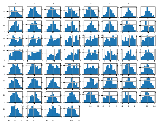

Train the model

df = read_csv(data_path + 'sonar.csv', header=None)

data = df.values

X, y = data[:, :-1], data[:, -1]

X = X.astype('float32')
y = LabelEncoder().fit_transform(y.astype('str'))

power = PowerTransformer(method='yeo-johnson')

model = KNeighborsClassifier()

pipeline = Pipeline(steps=[('p', power), ('m', model)])

cv = RepeatedStratifiedKFold(n_splits=10, n_repeats=3, random_state=1)

scores = cross_val_score(pipeline, X, y, scoring='accuracy', cv=cv)

print(f'Accuracy: {mean(scores): .3f}  {std(scores): .3f}')

Accuracy:  0.808   0.082

Sometimes a lift in performance can be achieved by first standardizing the raw dataset prior to performing a Yeo-Johnson transform. We can explore this by adding a StandardScaler as a first step in the pipeline. The complete example is listed below.

df = read_csv(data_path + 'sonar.csv', header=None)

data = df.values

X, y = data[:, :-1], data[:,-1]

X = X.astype('float32')
y = LabelEncoder().fit_transform(y.astype('str'))

scaler = StandardScaler()

power = PowerTransformer(method='yeo-johnson')

model = KNeighborsClassifier()

pipeline = Pipeline(steps=[('s', scaler), ('p', power), ('m', model)])

cv = RepeatedStratifiedKFold(n_splits=10, n_repeats=3, random_state=1)

scores = cross_val_score(pipeline, X, y, scoring='accuracy', cv=cv)

print(f'Accuracy: {mean(scores): .3f}, {std(scores): .3f}')

Accuracy:  0.816,  0.077

Change Numerical Data Distributions

Quantile Transforms

from sklearn.preprocessing import QuantileTransformer

data = randn(1000)

data = exp(data)

pyplot.hist(data, bins=25)
pyplot.show()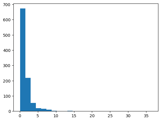

data = data.reshape(len(data), 1)

quantile = QuantileTransformer(output_distribution='normal')

data_trans = quantile.fit_transform(data)

pyplot.hist(data_trans, bins=25)
pyplot.show()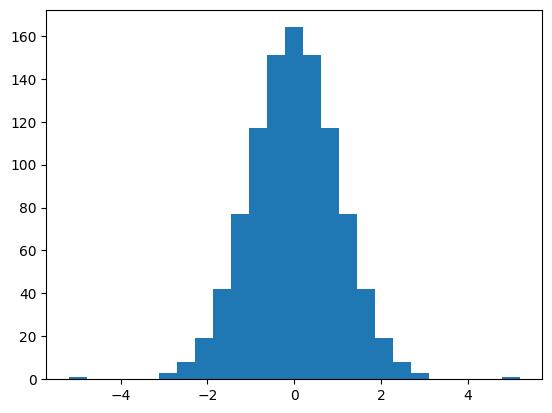

Sonar Dataset

df = read_csv(data_path + 'sonar.csv', header=None)

data = df.values[:, :-1]

trans = QuantileTransformer(n_quantiles=100, output_distribution='normal')

data = trans.fit_transform(data)

df = DataFrame(data)

fig = df.hist(xlabelsize=4, ylabelsize=4)
[x.title.set_size(4) for x in fig.ravel()]
pyplot.show()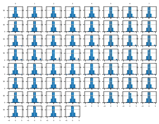

Next, let’s evaluate the same KNN model as the previous section, but in this case on a normal quantile transform of the dataset. The complete example is listed below.

df = read_csv(data_path + 'sonar.csv', header=None)

data = df.values

X, y = data[:, :-1], data[:, -1]

X = X.astype('float32')

y = LabelEncoder().fit_transform(y.astype('str'))

trans = QuantileTransformer(n_quantiles=100, output_distribution='normal')

model = KNeighborsClassifier()

pipeline = Pipeline(steps=[('t', trans), ('m', model)])

cv = RepeatedStratifiedKFold(n_splits=10, n_repeats=3, random_state=1)

scores = cross_val_score(pipeline, X, y, scoring='accuracy', cv=cv)

print(f'Accuracy: {mean(scores):.3f}  {std(scores): .3f}')

Accuracy: 0.817   0.087

Uniform Quantile Transform

df = read_csv(data_path + 'sonar.csv', header=None)

data = df.values[:, :-1]

trans = QuantileTransformer(n_quantiles=100, output_distribution='uniform')

data = trans.fit_transform(data)

df = DataFrame(data)

fig = df.hist(xlabelsize=4, ylabelsize=4)
[x.title.set_size(4) for x in fig.ravel()]
pyplot.show()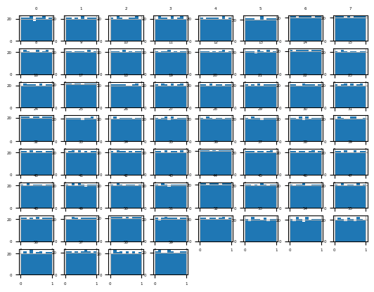

Next, let’s evaluate the same KNN model as the previous section, but in this case on a uniform quantile transform of the raw dataset.

df = read_csv(data_path + 'sonar.csv', header=None)

data = df.values

X, y = data[:, :-1], data[:, -1]

X = X.astype('float32')

y = LabelEncoder().fit_transform(y.astype('str'))

trans = QuantileTransformer(n_quantiles=100, output_distribution='uniform')

model = KNeighborsClassifier()

pipeline = Pipeline(steps=[('t', trans), ('m', model)])

cv = RepeatedStratifiedKFold(n_splits=10, n_repeats=3, random_state=1)

scores = cross_val_score(pipeline, X, y, scoring='accuracy', cv=cv)

print(f'Accuracy: {mean(scores):.3f}  {std(scores):.3f}')

Accuracy: 0.845  0.074

ed to explore the effect of the resolution of the transform on the resulting skill of the model. The example below performs this experiment and plots the mean accuracy for different n quantiles values from 1 to 99.

Transform Numerical to Categorical Data

from numpy.random import randn
from sklearn.preprocessing import KBinsDiscretizer
from matplotlib import pyplot

data = randn(1000)

pyplot.hist(data, bins=25)
pyplot.show()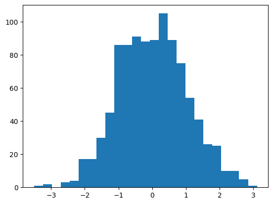

data = data.reshape(len(data), 1)

kbins = KBinsDiscretizer(n_bins=10, encode='ordinal', strategy='uniform')

data_trans = kbins.fit_transform(data)

print(data_trans[:10, :])

[[5.]
 [6.]
 [4.]
 [5.]
 [8.]
 [6.]
 [3.]
 [7.]
 [6.]
 [4.]]

pyplot.hist(data_trans, bins=10)
pyplot.show()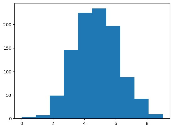

Sonar Dataset

from pandas import read_csv
from matplotlib import pyplot

df = read_csv(data_path + 'sonar.csv', header=None)

print(df.shape)

(208, 61)

df.describe()

	0	1	2	3	4	5	6	7	8	9	10	11	12	13	14	15	16	17	18	19	20	21	22	23	24	25	26	27	28	29	30	31	32	33	34	35	36	37	38	39	40	41	42	43	44	45	46	47	48	49	50	51	52	53	54	55	56	57	58	59
count	208.000000	208.000000	208.000000	208.000000	208.000000	208.000000	208.000000	208.000000	208.000000	208.000000	208.000000	208.000000	208.000000	208.000000	208.000000	208.000000	208.000000	208.000000	208.000000	208.000000	208.000000	208.000000	208.000000	208.000000	208.000000	208.000000	208.000000	208.000000	208.000000	208.000000	208.000000	208.000000	208.000000	208.000000	208.000000	208.000000	208.000000	208.000000	208.000000	208.000000	208.000000	208.000000	208.000000	208.000000	208.000000	208.000000	208.000000	208.000000	208.000000	208.000000	208.000000	208.000000	208.000000	208.000000	208.000000	208.000000	208.000000	208.000000	208.000000	208.000000
mean	0.029164	0.038437	0.043832	0.053892	0.075202	0.104570	0.121747	0.134799	0.178003	0.208259	0.236013	0.250221	0.273305	0.296568	0.320201	0.378487	0.415983	0.452318	0.504812	0.563047	0.609060	0.624275	0.646975	0.672654	0.675424	0.699866	0.702155	0.694024	0.642074	0.580928	0.504475	0.439040	0.417220	0.403233	0.392571	0.384848	0.363807	0.339657	0.325800	0.311207	0.289252	0.278293	0.246542	0.214075	0.197232	0.160631	0.122453	0.091424	0.051929	0.020424	0.016069	0.013420	0.010709	0.010941	0.009290	0.008222	0.007820	0.007949	0.007941	0.006507
std	0.022991	0.032960	0.038428	0.046528	0.055552	0.059105	0.061788	0.085152	0.118387	0.134416	0.132705	0.140072	0.140962	0.164474	0.205427	0.232650	0.263677	0.261529	0.257988	0.262653	0.257818	0.255883	0.250175	0.239116	0.244926	0.237228	0.245657	0.237189	0.240250	0.220749	0.213992	0.213237	0.206513	0.231242	0.259132	0.264121	0.239912	0.212973	0.199075	0.178662	0.171111	0.168728	0.138993	0.133291	0.151628	0.133938	0.086953	0.062417	0.035954	0.013665	0.012008	0.009634	0.007060	0.007301	0.007088	0.005736	0.005785	0.006470	0.006181	0.005031
min	0.001500	0.000600	0.001500	0.005800	0.006700	0.010200	0.003300	0.005500	0.007500	0.011300	0.028900	0.023600	0.018400	0.027300	0.003100	0.016200	0.034900	0.037500	0.049400	0.065600	0.051200	0.021900	0.056300	0.023900	0.024000	0.092100	0.048100	0.028400	0.014400	0.061300	0.048200	0.040400	0.047700	0.021200	0.022300	0.008000	0.035100	0.038300	0.037100	0.011700	0.036000	0.005600	0.000000	0.000000	0.000000	0.000000	0.000000	0.000000	0.000000	0.000000	0.000000	0.000800	0.000500	0.001000	0.000600	0.000400	0.000300	0.000300	0.000100	0.000600
25%	0.013350	0.016450	0.018950	0.024375	0.038050	0.067025	0.080900	0.080425	0.097025	0.111275	0.129250	0.133475	0.166125	0.175175	0.164625	0.196300	0.205850	0.242075	0.299075	0.350625	0.399725	0.406925	0.450225	0.540725	0.525800	0.544175	0.531900	0.534775	0.463700	0.411400	0.345550	0.281400	0.257875	0.217575	0.179375	0.154350	0.160100	0.174275	0.173975	0.186450	0.163100	0.158900	0.155200	0.126875	0.094475	0.068550	0.064250	0.045125	0.026350	0.011550	0.008425	0.007275	0.005075	0.005375	0.004150	0.004400	0.003700	0.003600	0.003675	0.003100
50%	0.022800	0.030800	0.034300	0.044050	0.062500	0.092150	0.106950	0.112100	0.152250	0.182400	0.224800	0.249050	0.263950	0.281100	0.281700	0.304700	0.308400	0.368300	0.434950	0.542500	0.617700	0.664900	0.699700	0.698500	0.721100	0.754500	0.745600	0.731900	0.680800	0.607150	0.490350	0.429600	0.391200	0.351050	0.312750	0.321150	0.306300	0.312700	0.283500	0.278050	0.259500	0.245100	0.222550	0.177700	0.148000	0.121350	0.101650	0.078100	0.044700	0.017900	0.013900	0.011400	0.009550	0.009300	0.007500	0.006850	0.005950	0.005800	0.006400	0.005300
75%	0.035550	0.047950	0.057950	0.064500	0.100275	0.134125	0.154000	0.169600	0.233425	0.268700	0.301650	0.331250	0.351250	0.386175	0.452925	0.535725	0.659425	0.679050	0.731400	0.809325	0.816975	0.831975	0.848575	0.872175	0.873725	0.893800	0.917100	0.900275	0.852125	0.735175	0.641950	0.580300	0.556125	0.596125	0.593350	0.556525	0.518900	0.440550	0.434900	0.424350	0.387525	0.384250	0.324525	0.271750	0.231550	0.200375	0.154425	0.120100	0.068525	0.025275	0.020825	0.016725	0.014900	0.014500	0.012100	0.010575	0.010425	0.010350	0.010325	0.008525
max	0.137100	0.233900	0.305900	0.426400	0.401000	0.382300	0.372900	0.459000	0.682800	0.710600	0.734200	0.706000	0.713100	0.997000	1.000000	0.998800	1.000000	1.000000	1.000000	1.000000	1.000000	1.000000	1.000000	1.000000	1.000000	1.000000	1.000000	1.000000	1.000000	1.000000	0.965700	0.930600	1.000000	0.964700	1.000000	1.000000	0.949700	1.000000	0.985700	0.929700	0.899500	0.824600	0.773300	0.776200	0.703400	0.729200	0.552200	0.333900	0.198100	0.082500	0.100400	0.070900	0.039000	0.035200	0.044700	0.039400	0.035500	0.044000	0.036400	0.043900

fig = df.hist(xlabelsize=4, ylabelsize=4)
[x.title.set_size(4) for x in fig.ravel()]
pyplot.show()

Let’s fit and evaluate a machine learning model on the raw dataset.

from numpy import mean, std
from sklearn.preprocessing import LabelEncoder
from sklearn.neighbors import KNeighborsClassifier
from sklearn.model_selection import RepeatedStratifiedKFold, cross_val_score

df = read_csv(data_path + 'sonar.csv', header=None)

data = df.values

X, y = data[:, :-1], data[:, -1]

X = X.astype('float32')
y = LabelEncoder().fit_transform(y.astype('str'))

model = KNeighborsClassifier()

cv = RepeatedStratifiedKFold(n_splits=10, n_repeats=3, random_state=1)

n_scores = cross_val_score(model, X, y, scoring='accuracy', cv=cv)

print(f'Accuracy: {mean(n_scores): .3f}, {std(n_scores): .3f}')

Accuracy:  0.797,  0.073

Uniform Discretization Transform

from pandas import DataFrame
from sklearn.pipeline import Pipeline

df = read_csv(data_path + 'sonar.csv', header=None)

data = df.values[:, :-1]

trans = KBinsDiscretizer(n_bins=10, encode='ordinal', strategy='uniform')

data = trans.fit_transform(data)

df = DataFrame(data)

fig = df.hist(xlabelsize=4, ylabelsize=4)
[x.title.set_size(4) for x in fig.ravel()]
pyplot.show()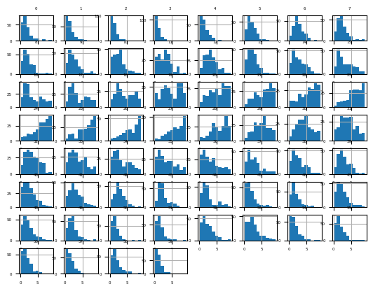

Next, let’s evaluate the same KNN model as the previous section

df = read_csv(data_path + 'sonar.csv', header=None)

data = df.values

X, y = data[:, :-1], data[:, -1]

X = X.astype('float32')
y = LabelEncoder().fit_transform(y.astype('str'))

trans = KBinsDiscretizer(n_bins=10, encode='ordinal', strategy='uniform')

model = KNeighborsClassifier()

pipeline = Pipeline(steps = [('t', trans), ('m', model)])

cv = RepeatedStratifiedKFold(n_splits=10, n_repeats=3, random_state=1)

n_scores = cross_val_score(pipeline, X, y, scoring='accuracy', cv=cv)

print(f'Accuracy: {mean(n_scores):.3f}, {std(n_scores):.3f}')

Accuracy: 0.829, 0.079

k-Means Discretization Transform

df = read_csv(data_path + 'sonar.csv', header=None)

data = df.values[:, :-1]

trans = KBinsDiscretizer(n_bins=3, encode='ordinal', strategy='kmeans')

data = trans.fit_transform(data)

df = DataFrame(data)

fig = df.hist(xlabelsize=4, ylabelsize=4)
[x.title.set_size(4) for x in fig.ravel()]
pyplot.show()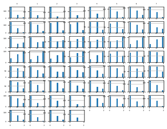

Next, let’s evaluate the same KNN model

df = read_csv(data_path + 'sonar.csv', header=None)

data = df.values

X, y = data[:, :-1], data[:, -1]

X = X.astype('float32')
y = LabelEncoder().fit_transform(y.astype('str'))

trans = KBinsDiscretizer(n_bins=3, encode='ordinal', strategy='kmeans')

model = KNeighborsClassifier()

pipeline = Pipeline(steps=[('t', trans), ('m', model)])

cv = RepeatedStratifiedKFold(n_splits=10, n_repeats=3, random_state=1)

n_scores = cross_val_score(pipeline, X, y, scoring='accuracy', cv=cv)

print(f'Accuracy: {mean(n_scores):.3f}, {std(n_scores):.3f}')

Accuracy: 0.814, 0.084

Quantile Discretization Transform

df = read_csv(data_path + 'sonar.csv', header=None)

data = df.values[:, :-1]

trans = KBinsDiscretizer(n_bins=10, encode='ordinal', strategy='quantile')

data = trans.fit_transform(data)

df = DataFrame(data)

fig = df.hist(xlabelsize=4, ylabelsize=4)
[x.title.set_size(4) for x in fig.ravel()]
pyplot.show()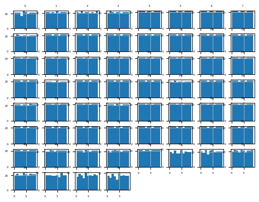

Next, let’s evaluate the same KNN model

df = read_csv(data_path + 'sonar.csv', header=None)

data = df.values

X, y = data[:, :-1], data[:, -1]

X = X.astype('float32')
y = LabelEncoder().fit_transform(y.astype('str'))

trans = KBinsDiscretizer(n_bins=10, encode='ordinal', strategy='quantile')

model = KNeighborsClassifier()

pipeline = Pipeline(steps=[('t', trans), ('m', model)])

cv = RepeatedStratifiedKFold(n_splits=10, n_repeats=3, random_state=1)

n_scores = cross_val_score(pipeline, X, y, scoring='accuracy', cv=cv)

print(f'Accuracy: {mean(n_scores):.3f} {std(n_scores): .3f}')

Accuracy: 0.840  0.072

We chose the number of bins as an arbitrary number; in this case, 10. This hyperparameter can be tuned to explore the effect of the resolution of the transform on the resulting skill of the model.

def get_dataset(filename):
    df = read_csv(filename, header=None)
    data = df.values
    X, y = data[:, :-1], data[:, -1]
    X = X.astype('float32')
    y = LabelEncoder().fit_transform(y.astype('str'))
    return X, y

def get_models():
    models = dict()
    for i in range(2, 11):
        trans = KBinsDiscretizer(n_bins=i, encode='ordinal', strategy='quantile')
        model = KNeighborsClassifier()
        models[str(i)] = Pipeline(steps=[('t', trans), ('m', model)])
    return models

def evaluate_model(model, X, y):
    cv = RepeatedStratifiedKFold(n_splits=10, n_repeats=3, random_state=1)
    scores = cross_val_score(model, X, y, scoring='accuracy', cv=cv)
    return scores

X, y = get_dataset()

models = get_models()

results, names = list(), list()

for name, model in models.items():
    scores = evaluate_model(model, X, y)
    results.append(scores)
    names.append(name)
    print(f'{name}: {mean(scores): .3f} {mean(scores): .3f}')

2:  0.822  0.822
3:  0.870  0.870
4:  0.838  0.838
5:  0.838  0.838
6:  0.844  0.844
7:  0.852  0.852
8:  0.838  0.838
9:  0.841  0.841
10:  0.840  0.840

pyplot.boxplot(results, labels=names, showmeans=True)
pyplot.show()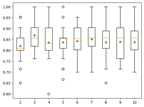

Derive New Input Variables

Polynomial Feature Transform

from numpy import asarray
from sklearn.preprocessing import PolynomialFeatures

data = asarray([[2,3], [2,3], [2,3]])
print(data)

[[2 3]
 [2 3]
 [2 3]]

trans = PolynomialFeatures(degree=2)

data = trans.fit_transform(data)

print(data)

[[1. 2. 3. 4. 6. 9.]
 [1. 2. 3. 4. 6. 9.]
 [1. 2. 3. 4. 6. 9.]]

Polynomial Feature Transform Example

df = read_csv(data_path + 'sonar.csv', header=None)

data = df.values[:, :-1]

trans = PolynomialFeatures(degree=3)

data = trans.fit_transform(data)

df = DataFrame(data)

print(df.shape)

(208, 39711)

Next, let’s evaluate the same KNN model

df = read_csv(data_path + 'sonar.csv', header=None)

data = df.values

X, y = data[:, :-1], data[:, -1]

X = X.astype('float32')

y = LabelEncoder().fit_transform(y.astype('str'))

trans = PolynomialFeatures(degree=3)

model = KNeighborsClassifier()

pipeline = Pipeline(steps=[('t', trans), ('m', model)])

cv = RepeatedStratifiedKFold(n_splits=10, n_repeats=3, random_state=1)

n_scores = cross_val_score(pipeline, X, y, scoring='accuracy', cv=cv)

print(f'Accuracy: {mean(n_scores):.3f} {std(n_scores): .3f}')

Accuracy: 0.800  0.077

Effect of Polynomial Degree

X, y = get_dataset(data_path + 'sonar.csv')

num_feature = list()

degrees = [i for i in range(1, 6)]

for d in degrees:
    trans = PolynomialFeatures(degree=d)
    data = trans.fit_transform(X)
    num_feature.append(data.shape[1])
    print(f'Degree: {d}, Features: {data.shape[1]}')

Degree: 1, Features: 61
Degree: 2, Features: 1891
Degree: 3, Features: 39711
Degree: 4, Features: 635376
Degree: 5, Features: 8259888

pyplot.plot(degrees, num_feature)
pyplot.show()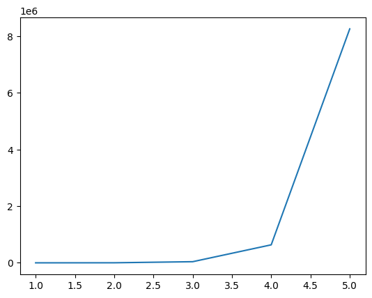

It may be a good idea to treat the degree for the polynomial features transform as a hyperparameter and test different values for your dataset.

def get_models():
    models = dict()
    for d in range(1,5):
        trans = PolynomialFeatures(degree=d)
        model = KNeighborsClassifier()
        models[str(d)] = Pipeline(steps=[('t', trans), ('m', model)])
    return models

X, y = get_dataset(data_path + 'sonar.csv')

models = get_models()

results, names = list(), list()

for name, model in models.items():
    scores = evaluate_model(model, X, y)
    results.append(scores)
    names.append(name)
    print(f'{name}: {mean(scores):.3f} {std(scores):.3f}')

1: 0.797 0.073
2: 0.793 0.085
3: 0.800 0.077
4: 0.795 0.079

pyplot.boxplot(results, labels=names, showmeans=True)
pyplot.show()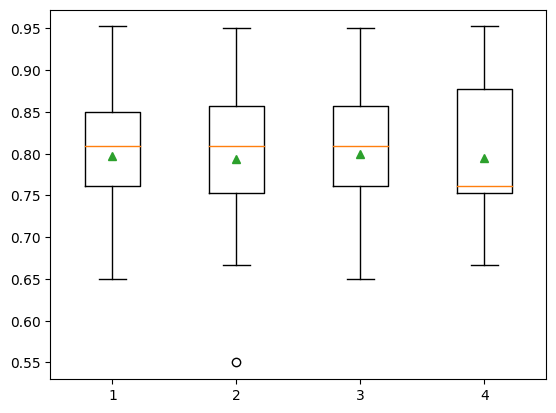

Advanced Transforms

Transform Both Numerical and Categorical Data

Data Preparation for the Abalone Regression Dataset

from numpy import absolute
from sklearn.preprocessing import OneHotEncoder, MinMaxScaler
from sklearn.compose import ColumnTransformer
from sklearn.svm import SVR
from sklearn.model_selection import KFold

df = read_csv(data_path + 'abalone.csv', header=None)

last_ix = len(df.columns) - 1

X, y = df.drop(last_ix, axis=1), df[last_ix]

print(X.shape, y.shape)

(4177, 8) (4177,)

numerical_ix = X.select_dtypes(include=['int64', 'float64']).columns
categorical_ix = X.select_dtypes(include=['object', 'bool']).columns

t = [('cat', OneHotEncoder(), categorical_ix), ('num', MinMaxScaler(), numerical_ix)]

col_transform = ColumnTransformer(transformers=t)

model = SVR(kernel='rbf', gamma = 'scale', C=100)

pipeline = Pipeline(steps=[('prep', col_transform), ('m', model)])

cv = KFold(n_splits=10, shuffle=True, random_state=1)

scores = cross_val_score(pipeline, X, y, scoring='neg_mean_absolute_error', cv=cv)

scores = absolute(scores)

print(f'MAE: {mean(scores):.3f} {std(scores): .3f}')

MAE: 1.465  0.047

Transform the Target in Regression

Example of Using the TransformedTargetRegressor

from numpy import loadtxt
from sklearn.linear_model import HuberRegressor
from sklearn.compose import TransformedTargetRegressor
from sklearn.model_selection import RepeatedKFold

data = loadtxt(data_path + 'boston-housing.csv')

X, y = data[:, :-1], data[:, -1]

pipeline = Pipeline(steps=[('normalize', MinMaxScaler()), ('model', HuberRegressor())])

model = TransformedTargetRegressor(regressor=pipeline, transformer=MinMaxScaler())

cv = RepeatedKFold(n_splits=10, n_repeats=3, random_state=1)

scores = cross_val_score(model, X, y, scoring='neg_mean_absolute_error', cv=cv)

scores=absolute(scores)

print(f'Mean: {mean(scores):.3f}')

Mean: 3.203

We are not restricted to using scaling objects; for example, we can also explore using other data transforms on the target variable, such as the PowerTransformer

from sklearn.preprocessing import PowerTransformer

data = loadtxt(data_path + 'boston-housing.csv')

X, y = data[:, :-1], data[:, -1]

steps = list()

steps.append(('scale', MinMaxScaler(feature_range=(1e-5, 1))))
steps.append(('power', PowerTransformer()))
steps.append(('model', HuberRegressor()))

pipeline = Pipeline(steps=steps)

model = TransformedTargetRegressor(regressor=pipeline, transformer=PowerTransformer())

cv = RepeatedKFold(n_splits=10, n_repeats=3, random_state=1)

scores = cross_val_score(model, X, y, scoring='neg_mean_absolute_error', cv=cv)

scores = absolute(scores)

print(f'Mean: {mean(scores): .3f}')

Mean:  2.972

How to Save and Load Data Transforms

Worked Example of Saving Data Preparatio

Define a Dataset

from sklearn.datasets import make_blobs
from sklearn.model_selection import train_test_split

X, y = make_blobs(n_samples=100, centers=2, n_features=2, random_state=1)

X_train, X_test, y_train, y_test = train_test_split(X, y, test_size=0.33, random_state=1)

for i in range(X_test.shape[1]):
    print(f'{i} > train: min={X_train[:, i].min():.3f}, max={X_train[:,i].max(): .3f}, test: min={X_test[:,i].min():.3f}, max={X_test[:,i].max():.3f}')

0 > train: min=-11.856, max= 0.526, test: min=-11.270, max=0.085
1 > train: min=-6.388, max= 6.507, test: min=-5.581, max=5.926

Scale the Dataset

from sklearn.linear_model import LogisticRegression
from pickle import dump

X, y = make_blobs(n_samples=100, centers=2, n_features=2, random_state=1)

X_train, X_test, y_train, y_test = train_test_split(X, y, test_size=0.33, random_state=1)

scaler = MinMaxScaler()

scaler.fit(X_train)

MinMaxScaler()

X_train_scaled = scaler.transform(X_train)

X_test_scaled = scaler.transform(X_test)

for i in range(X_test.shape[1]):
        print(f'{i} > train: min={X_train_scaled[:, i].min():.3f}, max={X_train_scaled[:,i].max(): .3f}, test: min={X_test_scaled[:,i].min():.3f}, max={X_test_scaled[:,i].max():.3f}')

0 > train: min=0.000, max= 1.000, test: min=0.047, max=0.964
1 > train: min=0.000, max= 1.000, test: min=0.063, max=0.955

Save Model and Data Scaler

X, y = make_blobs(n_samples=100, centers=2, n_features=2, random_state=1)

X_tarin, _, y_train, _ = train_test_split(X, y, test_size=0.33, random_state=1)

scaler = MinMaxScaler()

scaler.fit(X_tarin)

MinMaxScaler()

X_train_scaled = scaler.transform(X_train)

model = LogisticRegression(solver='lbfgs')

model.fit(X_train_scaled, y_train)

LogisticRegression()

dump(model, open('model.pkl', 'wb'))

dump(scaler, open('scaler.pkl', 'wb'))

Load Model and Data Scaler

from pickle import load

X, y = make_blobs(n_samples=100, centers=2, n_features=2, random_state=1)

_, X_test, _, y_test = train_test_split(X, y, test_size=0.33, random_state=1)

scaler = load(open('model.pkl'))